Unit III Lesson 8

Boundary Value Problems

Boundary value problems: deflection (bending under its own weight) of a beam as a fourth order boundary value problem.
Example of solving the fourth order boundary value problem, use of Cramer's rule.
Eigenvalues and Eigenfunctions of certain types of boundary value problems.
An example of use of Eigenvalues and Eigenfunctions applied to a structure, critical loads, 'buckling'.
Another example of a boundary value problem.
A 'show that' problem from thremodynamics.

The preceding lesson was about dynamic systems that were modeled by initial value problems. Often, however, the mathematical description of a physical system demands that we solve a DE that has ‘boundary conditions’. That means we know values of the function, one or more of its derivatives, or even some linear combination of the function and its derivatives at two or more points. Several such examples follow.

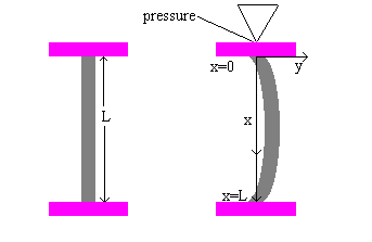
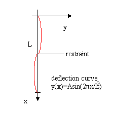
Deflection of a Beam

Many structures built by humans are constructed from girders or beams which deflect or distort (Shall we say bend?) under their own weight or due to some external force. This deflection is governed by a linear 4^th order DE. The diagram here shows the deflection curve of a beam:

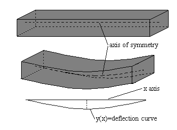
Suppose the x axis coincides with the axis of symmetry and the deflection is positive in a downward direction. In the theory of elasticity, it is known that the bending moment M(x) at a point x along the axis of the beam is related to the load per unit length w(x) by the DE:

In addition, the bending moment M(x)=EIk where E and I are constants and k is the curvature of the elastic curve. E involves the elasticity of the beam's material (Steel is more rigid than lead, for example) and I is the moment of inertia of a cross section of the beam about the ‘neutral axis’. The product EI is called the flexural rigidity of the beam.

You may recall from calculus class that curvature k is given by the formula:

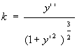When the deflection is small y’è 0 so the denominator è 1, so k=y’’ is used as the equation for curvature. Then M(x)=EIk can be written M(x)=EIy’’.

Differentiating this twice gives the DE.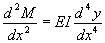

Since, the left side of the above equation replaced with w(x) would yield:.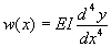

Boundary conditions associated with the equation depend on how the ends of the beam are supported. A cantilever beam is fixed at one end and free at the other end as the diagram shows:

For an embedded cantilever beam, the deflection y(x) must satisfy two boundary conditions at the embedded end and two at the free end:

y(0)=0 since there is no deflection at this end, and
y’(0)=0 since the deflection curve is tangent to the x axis at this end.
y’’(L)=0 (where L is the beam’s length) since the bending moment is zero at the end
y’’’(L)=0 since the shear force at the end is zero.

If the beam is simply hinged on the fixed end, then y(0)=0 and y’’(0)=0.

If the beam is embedded at both ends, there is no vertical deflection and the line of deflection is horizontal at the endpoints, which gives boundary conditions:

y(0)=0, y’(0)=0, y(L)=0, y’(L)=0. A picture of the situation is given:

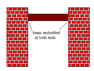
Ex1. A beam of length L is embedded at both ends, and the constant load w₀ is uniform along its length. (I.e. w(x)=w₀ for all x in the interval 0<x<L). Find the function representing the deflection of the beam.

Take this link after trying it yourself.

Eigenvalues and Eigenfunctions

Suppose we wish to solve the BVP y’’+cy=0 with y(0)=0 and y(L)=0.

Case 1 c=0

y’’=0 is the differential equation, so y’=A, y=Ax+B and y(0)=0 forces B=0, y(L)=0 forces AL=0 hence A=0, and we have only the trivial solution y=0

Case 2 c<0

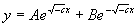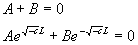
From the characteristic equation m²+c=0 (with c<0) we get the solutions . From the boundary values, we get the system of equations

If B=-A, (from the first equation) then the second equation says . Since L>0 and c<0, this forces A=-B=0 and we again have only the trivial solution y=0.

Case 3 c>0 we get the solution 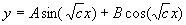. y(0)=0 forces B=0 and y(L)=0 means that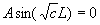. Here either A=0 or else . Solved for c, we get.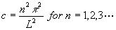

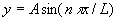
(Note if n=0, then c=0 and we already looked at that in Case 1. Hence is a solution for any A if .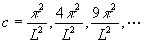

These values are called characteristic values or eigenvalues of the equation and the corresponding functions

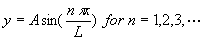
are called characteristic functions or eigenfunctions.

Real Life Example (you don’t have to work this one first!)

Consider a vertical column of length L hinged at both ends, with a constant vertical compressive force (pressure) P applied to its top. The boundary value problem governing its deflection y(x) is

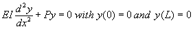
where E is a constant involving elasticity of the object’s material and I is the moment of inertia of a cross section about a vertical line through its centroid. Here is a picture of the situation:

By letting c=P/EI, we have the situation described previously:

y’’+cy=0 with y(0)=0 and y(L)=0

We either have y=0 as a deflection curve or we have Case 3 where

corresponding to eigenvalues

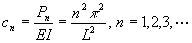
Therefore the column will buckle only if the pressure on the column is one of the values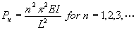. These forces are called critical loads.

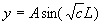
The deflection curve corresponding to the smallest critical load, called the Euler load ,is and is known as the first buckling mode.

If a restraint is placed on the column at x=L/2 (half-way point), then the smallest critical load will beand the deflection curve will be as in the figure shown here:

If restraints are placed at x=L/3 and x=2L/3, the critical load becomes

and so forth for other values of n.

Ex2. Find the eigenvalues and eigenfunctions for the given BVP:

Take this link after trying it yourself.

Ex3. The temperature u(r) in the circular ring shown below is determined from the boundary value problem: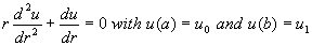

for u₀and u₁ constants.

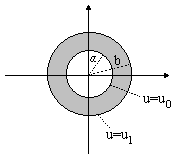
Show that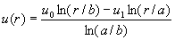

Take this link after trying it yourself.

****assignment****
Chapter 5 Section 2
Problems 1,5,9,27 Bonus for 7